Software Structure
We integrated a series of statistical analysis options in MetaComp (see Figure 1), ranging from descriptive multivariate statistical analyses, hypothesis testing analyses, nonlinear regression analysis of environmental factors and corresponded visualization. Herein, we introduce each statistical analysis option in the following paragraphs.

Figure 1: The workflow of MetaComp.
The input data of MetaComp include meta-omics data input (for all analyses) and environmental factors input (only for regression analysis). The analysis procedure in MetaComp consist of three independent parts: multivariate statistics (PCA and cluster analysis), statistical hypothesis tests (two-sample test, multi-sample test and two-group sample test) and regression analysis of environmental factors. The outputs are provided in Excel spreadsheet (k-means clustering results, statistically significance for each feature and regression analysis results) and visualized in diagrams (PCA map, hierarchical clustering dendrogram, bar plot, MDS map, heat-map).
Multivariate statistics
MetaComp employs principal component analysis (PCA) and clustering approaches (e.g.k-means clustering and hierarchical clustering) to present an overview of the differences among the given sets of meta-omics samples and highlight main features for each sample. Though it is a descriptive statistical function, these results are indispensable visualizations of meta-omics features. For example, enterotypes is illustrated by PCA figure.
Statistical hypothesis tests

where

and P = (ci1+ ci2)/(Ni1+Ni2). Sincez-test is not valid if the feature size is insufficient, the prerequisite ofz-test is min(ci1, ci2) ≤ zi2. When the sample size is small or user demands a more strict hypothesis testing method, MetaComp also offers Fisher��s exact test as an alteration (see the user guide of MetaComp for detailed recommendation).
Mode of multi-sample test: In this mode, pairwise tests between all conceivable pairs of samples are executed byz-test. Thep-value of a specific feature i is the minimum of all conceivablep-values. Thus we can identify that the selected feature is significantly different in at least one pair of samples.
Mode of two-group sample test: During this test, all samples are classified into two groups. In MetaComp, we provide four statistical hypothesis test methods (t-test, pairedt-test, Mann-Whitney U test and Wilcoxon signed-rank test) to assess whether a specific feature is significantly different between two groups of samples. Users can choose a proper method themselves or let MetaComp determine the most suitable test method according to the criterion shown in the following table.
If MetaComp judges that input data follow a Gaussian distribution, parametric hypothesis testing should be introduced. Otherwise when sample size is small or normality assumption is violated, nonparametric hypothesis testing should be conducted. If two groups of samples are consist of matched pairs for resemble units, or one group of units that has been tested twice, it indicates that two groups of samples are correlated. This automatical hypothesis testing selection will be helpful for users lacking of adequate statistical training.
Table 1: Criterion for selecting appropriate test.

Moreover, odds ratio (OR) test was also implemented to evaluate the relative abundance for each feature as the following table demonstrated. Here, G1and G2is in short for Group 1 and Group 2. cjkdenotes as counts for the j-th feature from the k-th group samples. Considering the possibility of unevenness between two groups, an empirical continuity correction has been introduced to improve the accuracy of the test. Consequently, OR statistic for feature i is

Where R = M1/M2. According to the formula above, features are categorized as group 1 enrichment (when log2OR(i) > 1) or group 1 scarcity (when log2OR(i) < 1).
Table 2: Contengency table for odd ratio test.

Multiple test correction
As the typical meta-omics profile consists of hundreds to thousands of features (e.g. Pfam/COG functional profiles), direct application of statistical method described above may probably lead to large numbers of false positives. For example, choosing a threshold of 0.05 will introduce 500 false positives in a profile contains 10000 features. Therefore, two correction methods are implemented in the MetaComp software to solve this problem, including false discovery rate (FDR) as the default option and a stricter option Bonferroni correction.
Regression analysis of environmental factors
MetaComp provides a novel function, regression analysis of environmental factors, which means regression analysis of the influence exerted by environmental factors on microbial communities. This original function is implemented by nonlinear regression analysis via the lasso algorithm. MetaComp first normalizes the data of both meta-omics samples and environmental factors. After that, the i-th environmental factor in j-th sample (which we shall denote by xij) is considered as independent variable, and the j-th frequency of k-th feature (which we shall denote by ykj) is considered as dependent variable. Therefore, the regression function is:

where xmj· xnjmeans the co-effect of environmental factor xmjand xnjto feature ykj. Then, αkiand βkmnrepresent the regression coefficient of the function. For any specific feature, the influence of environmental factors on samples is appraised by coefficient value and correlation value. Moreover, the reliability of the regression coefficient is determined byp-value. Only when allp-values meet the prescribed standard, the result of regression would be accepted by MetaComp.
Visualization of statistical significance analysis
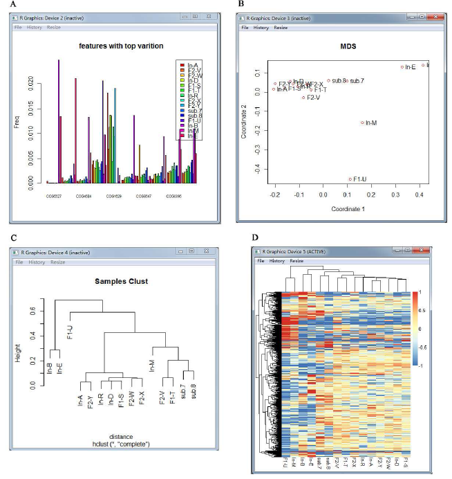
Figure 2: Visualizations of Statistical analyses.
(A) The bar plot of the top ten significantly different features. (B) The multi-dimensional scaling map of samples. Each point represents an individual sample. (C) The hierarchical clustering dendrogram of given samples.(D) The heat-map of given metagenomic samples.
For the MetaComp software, the visualizations of the hypothesis testing results are displayed in Figure 2, including:
Bar plot: Bar plot is exhibited for the top 10 significantly different features with their frequencies in each sample.
Hierarchical clustering dendrogram and multi-dimensional scaling map: Hierarchical clustering dendrogram and multi-dimensional scaling map are presented to illustrate the clustering and distance information of meta-omics samples respectively. Features with significant differences (p< 0.05) are involved in this clustering.
Two-dimensional heat-map: Two-dimensional heatmap is performed to investigate the relative abundance of each feature and the similarity among independent samples.
Moreover, our software enables to save the figures in many formats (e.g. .eps, .pdf, .png and .jpeg etc.) that can be used directly for publication.
Download List
Windows version installer of MetaCompMetaComp 1.1 version for Windows
Linux version package of MetaCompMetaComp 1.1 version for Linux
User guide for MetaCompUser Guide
Examples of standard input files for MetaCompStandard input
Additional files for the examples of MetaComp applicationAdditional files
Windows Version of MetaComp
The setup program is provided as msi file. MetaComp can be installed in any proper directory and then work for further analysis. Any further questions about installation of MetaComp, please refer to the installation instructions demonstrated in user guide.
Linux Version of MetaComp
The package of Linux version includes the following files:
MetaComp.R: R source codes of MetaComp.
Annotation.RData: An annotation for source codes of MetaComp.
User Guide for MetaComp
The detailed user guide in pdf format is provided. If you prefer an online version, please turn to user guide online for more information. User guide presents instructions on prerequisites and installation, formation of input data, and oprations for multivariate statistics, hypothesis testing and nonlinear regression analysis of environmental factors.
Examples of Standard Input Files
This package includes files as follows:
Standard input file in abundance profile matrix format:APM.txt
Two standard input files of BLAST(outfmt 7 format):Blast1.datand Blast2.dat
Two standard input files of HMMER:HMMER1.datand HMMER2.dat
Two standard input files of Kraken:Kraken1.datand Kraken2.dat
Standard input file of MG-RAST:MGRAST.tsv
Two standard input files of PhymmBL:phymmBL1.txtand phymmBL2.txt
Two standard input files of MZmine:MZ1.csvand MZ2.csv
Standardclustering informationinput for Mutivariate Statistical Analysis.
Inputs and results for the examples of MetaComp application
This package includes files as follows:
Additional file 1: The input functional gene APM data of eight typical environmental metagenomic samples. (txt 291 kb)
Additional file 2: The detailed analysis results of eight typical environmental metagenomic samples. (xls 2119 kb)
Additional file 3: The input functional gene APM data of Acid Mine Drainage metaproteomic samples. (xls 83kb)
Additional file 4: The detailed analysis results of Acid Mine Drainage metaproteomic samples. (xls 132 kb)
Additional file 5: The input metabolite APM data of human fecal sample from healthy control people and NAFLD patients. (xls 41kb)
Additional file 6: The detailed analysis results of human fecal sample from healthy control people and NAFLD patients. (xls 51kb)
Additional file 7: The input functional gene APM data of Hawaii Ocean metagenomic samples. (txt 72kb)
Additional file 8: The input vector of environmental factors related with Hawaii Ocean metagenomic samples. (txt 1 kb)
Additional file 9: The detailed analysis results of Hawaii Ocean metagenomic samples. (xls 50kb)
Additional file 10: The input functional gene APM data of Acid Mine Drainage metagenomic samples. (txt 62 kb)
Additional file 11: The input vector of environmental factors related with Acid Mine Drainage metagenomic samples. (txt 1 kb)
Additional file 12: The detailed analysis results of Acid Mine Drainage metagenomic samples. (xls 43 kb)
Additional file 13: The original, resampled and downsampled datasets of twin gut data for comparison of significance detection. (xls 622 kb)
Additional file 14: The hypothesis testing results of t-test, paired t-test, non-parametric t-test, Wilcoxon rank-sum test and Wilcoxon signed-rank test. (xls 168 kb)
Additional file 15: Visualized analysis results for Acid Mine Drainage metaproteomic samples and human fecal metabolomic samples. (pdf 204kb)
User Guide
1 Introduction
MetaComp is a graphical software for analyzing meta-omic (i.e. metagenomics, metatranscriptomics, metaproteomics and metabolomics) profiles with related environmental information, such as phylogenetic profiles indicating the number of marker genes assigned to different taxonomic units or functional profiles indicating the number of sequences assigned to different subsystems or pathways. The aim of this document provide an easy but comprehensive introduction to MetaComp and show how it can be used to analyze meta-omic data. MetaComp is applicable to any meta-omics data by accepting abundance profile matrices (APM) saved as txt or BIOM format files [1]. Moreover, MetaComp can autmatically converts the output of several widely used platform into MetaComp-compatible input file.
2 Prerequisites
Windows 7 or higher version.
Install Microsoft Office Excel 2010 or higher 64 bit version.
Install the required R packages using the following commands in the R console: install.packages("pheatmap").
3 MetaComp Installation
Windows: Download file "MetaComp setup.msi" setup from our website: http://cqb.pku.edu.cn/ZhuLab/MetaComp/download.html.
Linux: Download file "MetaComp.tar.gz" setup from our website: http://cqb.pku.edu.cn/ZhuLab/MetaComp/download.html. Enter the following commands: source(".//MetaComp.R").
4 Input data
4.1 Abundance profile matrix data
MetaComp reads input file in text format, and the values in the file should be separated by tab. The first row of the file shows the name of samples, while the first column represents the selected statistical feature. The cell of the table indicates the hit number of one sample to the given feature. Users must selectAbundance profile matrix (.txt or .biom)radio button fromProfiledialog box inLoad Dataoption withinFilemenu before choose the input profile. Moreover, the .biom format input must be convert to biom.table format before loading.(Figure 1-3) This format of input is the only format that can be load in Linux version. The command line is as follow:
input data = readFeature(file pathway, featuretype = "pfam" or "cog", format = "txt" or "biom")
Standard inputof APM form is provided.
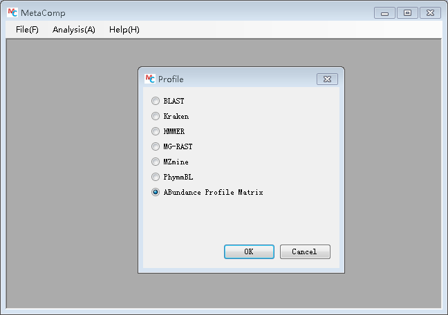
Figure 1: Choose APM as input.

Figure 2: Enter APM file either as .txt or .biom.

Figure 3: After APM data loaded.
4.2 Obtain profile from BLAST
MetaComp also accepts meta-omics profiles obtained from BLAST ([2], https://blast.ncbi.nlm.nih.gov/Blast.cgi) result. MetaComp works directly with BLAST result obtained by clicking on download in result web page, followed by selecting Hit Table(text) output type choice. Moreover, the BLAST result file can be obtained from table format (-outfmt 7). MetaComp can convert these BLAST results to standard Abundance profile matrices (APM) data through selectingBLASTradio button fromProfiledialog box inLoad Dataoption withinFilemenu. After opening up theBLASTdialog box, you can select the BLAST result files you wish to input. (Figure 4-6)
Standard inputof BLAST form is provided.

Figure 4: Choose BLAST result as input.

Figure 5: Enter BLAST result file directory.

Figure 6: After BLAST data loaded.
4.3 Obtain profile from HMMER
The input profile can also be acquired from HMMER ([3], http://hmmer.org/). Afterhmmer-3.1b2.tar.gzdownloaded and unpacked, you can get the desired results fromhmmsearchcommand. MetaComp can convert these file into MetaComp-compatible profiles through selectingHMMERradio button convert these BLAST results to standard Abundance profile matrices (APM) data through selectingBLASTradio button fromProfiledialog box inLoad Dataoption withinFilemenu. Click on theOKbutton after selecting the result file you wish to convert. (Figure 7-9)
Standard inputof HMMER output is provided.

Figure 7: Choose HMMER result as input.

Figure 8: Enter HMMER result file directory.

Figure 9: After HMMER data loaded.
4.4 Obtain profile from Kraken
Kraken ([4], http://ccb.jhu.edu/software/kraken/) result files are achieved from kraken-translate command. The selection of Kraken result file can initiate after choosingKrakenradio button fromProfiledialog box inLoad Dataoption withinFilemenu. (Figure 10-12)
Standard inputof Kraken output is provided.

Figure 10: Choose Kraken result as input.

Figure 11: Enter Kraken result file directory.

Figure 12: After Kraken data loaded.
4.5 Obtain profile from MG-RAST
MetaComp provides support for analyzing MG-RAST taxonomic or functional profiles. Visit the MG-RAST website ([5], http://metagenomics.anl.gov/) and browse the list of pubic metagenomes. Profiles for multiple samples can be obtained and downloaded as tab-separated values (tsv) file using the table data visualization. To work with MG-RAST profiles, they must be converted into a MetaComp-compatible profile. From within MetaComp, select theMG-RASTradio button fromProfiledialog box inLoad Dataoption withinFilemenu. This opens up theMG-RASTdialog box. Click on theOKbutton after selecting the MG-RAST profile you wish to convert. (Figure 13-15)
Standard inputof MG-RAST output form is provided.

Figure 13: Choose MG-RAST result as input.

Figure 14: Enter MG-RAST result file directory.

Figure 15: After MG-RAST data loaded.
4.6 Obtain profile from PhymmBL
PhymmBL([6], http://www.cbcb.umd.edu/software/phymm/) result files are achieved fromscoreReads.plcommand. The selection of PhymmBL result file can initiate after choosingPhymmBLradio button fromProfiledialog box inLoad Dataoption withinFilemenu. (Figure 16-18)
Standard inputof PhymmBL output is provided.

Figure 16: Choose PhymmBL result as input.

Figure 17: Enter PhymmBL result file directory.

Figure 18: After PhymmBL data loaded.
4.7 Obtain profile from MZmine
MZmine([7], http://mzmine.github.io/) result files are achieved as Figure 19. The selection of MZmine result file can initiate after choosingMZmineradio button fromProfiledialog box inLoad Dataoption within File menu.(Figure 20-22)
Standard inputof MZmine output is provided.

Figure 19: MZmine export selection.

Figure 20: Choose MZmine result as input.

Figure 21: Enter MZmine result file directory.

Figure 22: After MZmine data loaded.
5 Multivariate statistics
5.1 Cluster analysis
Cluster analysis can be perform in two model: K-means clustering and hierarchical clustering. K-means clustering model requires users to input the cluster number. Cluster analysis can be operate through theClustering analysisdialog inAnalysismenu.(Figure 23-26)
Linux commands line:
Hcluster(input data)(for hierarchical clustering)
KMeans(input data,cluster number)(fork-means clustering)

Figure 23: Choose Cluster analysis function.

Figure 24: Enter the number of groups (k) fork-means clustering.

Figure 25: Result ofk-means cluster.

Figure 26: Result of hiearchical clustering.
5.2 Principal component analysis
Principal component analysis (PCA) is applied in two model: whole data analysis model and clustering analysis model. Whole data analysis model is the model we common used. Also, clustering analysis model can apply PCA within the clustering information.The example of clustering information can be download from PCA can be applied through thePrincipal component analysisdialog inAnalysismenu.(Figure 27-29)
Linux commands line:
PCA(input data,ShowsampleName="text" or "NA")
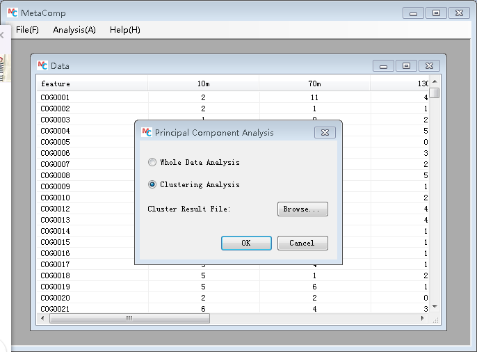
Figure 27: Choose a PCA mode from whole data analysis or clustering analysis.

Figure 28: Result of whole data PCA.

Figure 29: Result of clustering PCA.
6 Hypothesis testing
6.1 Two-sample test
To analyze a pair of samples, click on theTwo samples Statisticdialog inAnalysismenu. In this dialog, you can choose a favorable statistical test,p-value and data type. Moreover, you can choose the database you require if the feature in your profile is Pfam or COG database.(Figure 30-32)
Linux commands line:
result=twoSamplesComp(input data)
lotTopVar(result)

Figure 30: Two-sample test selection interface.

Figure 31: Detail result of two-sample test exported in Excel.

Figure 32: Bar plot for top ten significant differential features according to two-sample test.
6.2 Multi-sample test
To analyze multiple samples (more than two samples), click on theMultiple samples Statisticdialog inAnalysismenu. In this dialog, you can choose a favorable statistical test,p-value and data type. Just like two-sample test, you can choose the database you require if the feature in your profile is Pfam or COG database.(Figure 33-35)
Linux commands line:
result=twoSamplesComp(input data)
plotTopVar(result)
plotClust(result)
plotMDS(result)
plotHeatMap(input data)

Figure 33: Multi-sample test selection interface.

Figure 34: Detail result of multi-sample test exported in Excel.

Figure 35: Visualized analysis result for multi-sample test, from left to right: heatmap, multi-dimensional scaling (MDS), hiearchical clustering and bar plot for top ten significant differential features.
6.3 Two-group sample test
To analyze two group of samples, click on theTwo group of samples Statisticdialog inAnalysismenu. In this dialog, you can choose a favorable statistical test, group number andp-value. Meanwhile, you can chooseI do not knowoption inStatistics Methodcombo box while you do not know which method is the most suitable statistics test according to you input profile. Also, you can choose the database you require if the feature in your profile is Pfam or COG database.(Figure 36-38)
Linux commands line:
result=twoSamplesComp(input data,groupsep)(groupsep represents the sample number in first group.)
plotTopVar(result)
plotClust(result)
plotMDS(result)
plotHeatMap(input data)

Figure 36: Two-group sample test selection interface.

Figure 37: Detail result of two-group sample test exported in Excel.

Figure 38: Visualized analysis result for two-group sample test, from left to right: heatmap, multi-dimensional scaling (MDS), hiearchical clustering and bar plot for top ten significant differential features.
7 Environmental factors analysis
To operate environmental factors analysis, click on theEnvironmental factorsanalysis dialog inAnalysismenu. In this dialog, you need to load the environmental factors information, input thep-value, choose whether you require to include the cross term of environmental factors and load Pfam or COG database while analysing. The example of environmental factors information can be download from.(Figure 39-40)
Linux commands line:
EnvironmentFactor(input data,environment factor file pathway,Feature number)

Figure 39: Environmental factor analysis input.png.

Figure 40: Environmental factor analysis result.
References
1. Daniel McDonald, Jose C Clemente, Justin Kuczynski, Jai Ram Rideout, Jesse Stombaugh, Doug Wendel, Andreas Wilke, Susan Huse, John Hufnagle, Folker Meyer, et al. The biological observation matrix (biom) format or: how i learned to stop worrying and love the ome-ome. GigaScience, 1(1):1, 2012.
2. Stephen F Altschul, Warren Gish, Webb Miller, Eugene W Myers, and David J Lipman. Basic local alignment search tool. Journal of molecular biology, 215(3):403-10, 1990.
3. Jaina Mistry, Robert D Finn, Sean R Eddy, Alex Bateman, and Marco Punta. Challenges in homology search: Hmmer3 and convergent evolution of coiled-coil regions. Nucleic acids research, 41(12):e121-e121, 2013.
4. Derrick E Wood and Steven L Salzberg. Kraken: ultrafast metagenomic sequence classification using exact alignments. Genome biology, 15(3):1, 2014.
5. Elizabeth M Glass, Jared Wilkening, Andreas Wilke, Dionysios Antonopoulos, and Folker Meyer. Using the metagenomics rast server (mg-rast) for analyzing shotgun metagenomes. Cold Spring Harbor Protocols, 2010(1):pdbprot5368, 2010.
6. Arthur Brady and Steven L Salzberg. Phymm and phymmbl: metagenomic phylogenetic classification with interpolated markov models. Nature methods, 6(9):673-76, 2009.
7. Tomas Pluskal, Sandra Castillo, Alejandro Villar-Briones, and Matej Oresic. Mzmine 2: Modular framework for processing, visualizing, and analyzing mass spectrometry-based molecular profile data. BMC Bioinformatics, 11(1):395, 2010.
Application Examples
Comparative analysis of eight typical environmental metagenomic samples
Table 1: Part of whale fall, Acid Mine Drainage, Sargasso Sea, and Minnesota soil metagenomic samples analysis result.


Figure 1: Visualizations of metagenomic samples analysing results.
(A) This bar plot displays the top ten significantly different protein families among eight given samples. The frequencies of PF00072, PF00144, PF00872 in eight samples are dramatically fluctuated. (B) Hierarchical clustering dendrogram of eight given samples. (C) Multi-dimensional scaling map of eight given samples. Obviously, three samples from Sargasso Sea as well as three whale fall samples are grouped respectively; Minnesota farm soil and AMD samples are separated from Sargasso Sea samples and whale fall samples in both phylogenetic view and multi-dimensional distance. (D) The heat-map of eight given samples. This figure demonstrates our conclusion mentioned above through the similarity of relative gene abundance among eight samples.
Herein we analysed eight typical environmental metagenomic samples, including whale fall, Sargasso Sea, Minnesota farm soil and AMD, which were originally compared by Tringe et al. [1] (seeAdditional file 1for more details). The input shotgun sequenced data was annotated by Pfam database. Though amplicon sequenced 16s rRNA data was not included in this example, the processing was all the same as for shotgun sequenced metagenomic data. So that we only focused on comparing shotgun sequenced data in this case. During this analysis, we chose multi-sample test and the results clearly illustrate that the protein family profile of a microbial community is similar to that of other communities when their living environments are highly analogous (illustrated in Figure 1). According to the detailed analysis demonstrated inAdditional file 2, 3,456 protein families are significantly different (FDR < 0.01) among all given 11,110 compared protein families. These different features are closely related to the living conditions of metagenomic samples. For example, a large amount of bacteriorhodopsin-like proteins (e.g. PF01036) are found in all three Sargasso Sea samples, while these proteins are hardly detected in other samples. This protein is involved in obtaining light energy. In addition, since the content of potassium is apparently higher in AMD and soil, the quantity of potassium ion channel protein (e.g. PF03814, PF02705) in AMD and Minnesota farm soil greatly surpasses that in other samples (shown in Table 1).
References
1. Tringe, S.G., von Mering, C., Kobayashi, A., Salamov, A.A., Chen, K., Chang, H.W.: Comparative metagenomics of microbial communities. Science 308, 554-57 (2005)
Application Examples
Comparative analysis of Acid Mine Drainage metaproteomic samples
Table 1: Part of early and intermediate stage gene analysis result.

Due to similarity on characterizing dynamics of functional gene expression in a microbiota, it is enough to choose either metatranscriptomic samples or metaproteomic samples to test MetaComp performance. We then take metaproteomic samples of membrane and cytoplasmic proteins from biofilms at B-drift site of Richmond mine as input data for MetaComp. The biofilms were classified into early (labeled as GS0), intermediate (labeled as GS1) and late (labeled as GS2) growth stages. Significantly correlated proteins were identified by significance analysis of microarrays (SAM) or clustered by self-organizing tree algorithm (SOTA) in previous study (seeAdditional file 3: Table S3 for more details) [1]. Since MetaComp is designed for count data which means no negative variables is allowed as input, we transformed the original relative abundance data exponentially, with the base as 10.
Herein, we conducted two-sample z-test for these three samples. The results agree with the previous classification in most cases. For instance, 91.9% of early growth stage, 93.2% of late growth stage and 83.3% of intermediate growth stage expressed genes identified either by SAM or SOTA are also recognized by MetaComp. In addition, the rest proteins cannot provide comparing result due to too low abundance among compared samples.
We further observed that abundance of 65 out of 144 proteins identified previously as early stage expressed demonstrate significantly lower (p< 0.05) in early growth stage than intermediate stage. Meanwhile, previously identified intermediate stage expressed proteins indicate ap-value less than or equal to 4.18e-30. With thisp-value as threshold, 19 proteins still express significantly larger in intermediate stage than early stage, within which 10 proteins are engaged in environmental sensing procedure, others also correspond with specific cell processing and metabolic processing (seeAdditional file 4andAdditional file 15: Figure S1 to S3for more information). For example, LeptoII_Cont_10776_GENE_10 annotated as an important heat shock protein--GroEL, is regulated by RNA polymerase subunit sigma 32 during heat stress [2]. LeptoII_Scaffold_8241_GENE_340 annotated as Acetyl-CoA synthetase is also demanded in stationary phase rather than exponential phase to reduce fatty acids generated from membrane lipids [3]. Moreover, flagella synthesis related proteins (LeptoII_Scaffold_8241_GENE_209 annotated as FlgD, LeptoII_Scaffold_8241_GENE_653 annotated as FliD and LeptoII_Scaffold_7904_GENE_5 annotated as FlhA) are classified as intermediate expressed protein by MetaComp. According to the previous results [1], other flagellar proteins are expressed during intermediate and late stages of growth. We further noticed that LeptoII_Scaffold_8241_GENE_209, LeptoII_Scaffold_8241_GENE_653 and LeptoII_Scaffold_7904_GENE_5 only take parts in middle procedures of flagella biosynthesis other than from the beginning procedures [4]. Therefore, these genes identified as mainly expressed in intermediate stage by MetaComp is reasonable (these genes are listed in Table 1).
References
1. Mueller, R.S., Dill, B.D., Pan, C., Belnap, C.P., Thomas, B.C., VerBerkmoes, N.C., Hettich, R.L., Banfield, J.F.: Proteome changes in the initial bacterial colonist during ecological succession in an acid mine drainage biofilm community. Environ. Microbiol. 13(8), 2279-292 (2011)
2. Schumann, W.: Regulation of bacterial heat shock stimulons. Cell Stress Chaperones 21(6), 959-68 (2016)
3. Nystrom, T.: Stationary-phase physiology. Annu. Rev. Microbiol. 58, 161-81 (2004)
4. Macnab, R.M.: Genetics and biogenesis of bacterial flagella. Annu. Rev. Genet. 26(1), 131-58 (1992)
Application Examples
Comparative analysis of human fecal metabolomic samples
Table 1: Part of nonalcoholic fatty liver samples analysis results.

Since metabolome data indirectly reflect the conditional response of a microbial community, which is distinct with metatranscriptome and metaproteome, it is necessary to examine the performance of MetaComp on this data. We applied MetaComp on metabolomics data of fecal microbiota detected by Ramanet. al.[1]. The original data includes two groups of samples: 30 NAFLD patients for one group and another group with an equal number of healthy volunteers(seeAdditional file 5for more information). In Raman'study, researchers focused on detecting volatile organic compounds (VOC) which may exert toxic effect to human liver and secreted by human gut microbiota [1]. VOCs were not quantitatively measured but counted by detected or not per individual. Therefore, by gathering this binary counts for both prevalence group and control group, the maximum value for each type of VOC per group is 30.
MetaComp conducted a two-samplez-test on NAFLD and control group, and results indicate that 15 out of 220 VOCs are significantly different between two groups (seeAdditional file 6andAdditional file 15: Figure S4for more information). Furthermore, most VOCs identified as significantly different are included in previous study expect indolizine and acetic acid butyl ester and it may because of lacking of hits (only 5 hits in appeared in healthy control samples) that makes it difficult to be detected in previous study. It is notable that 6 out of 8 VOCs enriched in NAFLD fecal samples are short fatty acid esters. These derivatives of short fatty acids reflect that a relatively high concentration of hexose dietary such as frequently drinking soft drinks with fructose, which is a cause of NAFLD (shown in Table 1)[2].
References
1. Raman, M., Ahmed, I., Gillevet, P.M., Probert, C.S., Ratcliffe, N.M., Smith, S., Greenwood, R., Sikaroodi, M., Lam, V., Crotty, P., et al.: Fecal microbiome and volatile organic compound metabolome in obese humans with nonalcoholic fatty liver disease. Clin. Gastroenterol. Hepatol. 11(7), 868-75 (2013)
2. Nseir, W., Nassar, F., Assy, N.: Soft drinks consumption and nonalcoholic fatty liver. World J. Gastroenterol. 16(21), 2579-588 (2010)
Application Examples
Environmental factor analysis on Hawaii Ocean metagenomic samples

Figure 1: Diagrams of regression.
These diagrams exhibit the relationship between DIP and selected functional genes categorized by COG (COG0379, COG0458, COG0486, COG0849, COG1190 and COG1921). It is obviously that the abundance of these genes is linear with the content of DIP.
Table 1: Part of relationship between metagenomic samples and environmental factors analysis result.

We applied the novel function of MetaComp, regression analysis of environmental factors, on metagenomic samples from Hawaii Ocean [1] (seeAdditional file 7for more details). The input reads were aligned against COG database [2]. The selected environmental factors are dissolved inorganic phosphate (DIP) and oxygen content (OC) (seeAdditional file 8for more details). Concluded from the detailed analysis results (seeAdditional file 9for more details), we discover 102 out of 4,873 COGs which are probably corresponding to the living environment of Hawaii Ocean (p< 0.1). Moreover, some of the selected COG features are related to the generation and consumption of Adenosine Triphosphate (ATP), which is evidently related to phosphate and oxygen. For instance, COG0378, as a Ni2+-binding GTPase involved in regulation of expression and maturation of urease and hydrogenase, will generate organic phosphorus as well as dehydrogenase. Moreover, this reaction may consume oxygen. It is obvious that this COG is linked to both DIP and OC. Details of these protein families are shown in Table 1. Meanwhile, COGs relevant to the content of DIP (e.g. COG0379, COG0458, COG0486, COG0849, COG1190 and COG1921) are selected by MetaComp (illustrated in Figure 1).
References
1. DeLong, E.F., Preston, C.M., Mincer, T., Rich, V., Hallam, S.J., Frigaard, N.: Community genomics among stratified microbial assemblages in the ocean's interior. Science 311, 496-503 (2006)
2. Galperin, M.Y., Makarova, K.S., Wolf, Y.I., Koonin, E.V.: Expanded microbial genome coverage and improved protein family annotation in the cog database. Nucleic Acids Res. 43, 261-69 (2015)
Application Examples
Environmental factor analysis on Acid Mine Drainage metagenomic samples
A total of 40 AMD samples that varies in environmental characteristics were previously collected across Southeast China. Sampling procedure and data processing were described previously [1] (Additional file 10for more details). The measured environmental factors were dissolved oxygen (DO), total organic carbon (TOC) and SO42-(seeAdditional file 11for more details). According to the detailed analysis results (seeAdditional file 12files for more details), we discover 69 out of 142 genes which are presumably related to the living environment (p< 0.1). Among the selected genes, fumarate and nitrate reductase (fnr) gene is related to the respiratory chain of bacteria and the reaction of it requires a mass of sulfur. Therefore the abundance of fnr is apparently linked to DO and SO42-. Furthermore, ammonia monooxygenase A (amoA) is an enzyme, which catalyses nitration reaction. This reaction may consume organic carbon and oxygen. It is manifestly related to the content of TOC and DO.
1. Kuang, J., Huang, L., He, Z., Chen, L., Hua, Z., P, J., et al.: Predicting taxonomic and functional structure of microbial communities in acid mine drainage. ISME J. 10, 1527-39 (2016)
Application Examples
Evaluation on ability of differentially abundant features detection

Figure 1: ROC curve for all five methods.ROC performance of five methods in significant feature detection.
Table 1: Comparison of two-group sample test methods (FDR < 0.05)

Variations embedded in meta-omics are always difficult to recognize when the hit number of a feature is slightly different from one group of samples to another but evidently fluctuated among samples of the same group. Since that, to evaluate the differentially abundant features detection ability of current comparative meta-omics methods, we simulated two groups of count data from twin gut samples [1], of which 1,649,149 hits for 1,000 COG features was annotated through BLAST against COG database, to reserve the complexity of true data. Then we take a previous evaluation study for reference [2], samples are first amplified with fold change q = 1.25 and resampled into two equal sized groups of samples through randomly sampling without replacement. After that, 10% of COGs from the second group were chosen by chance and downsampled according to binomial distribution. Herein, we denoted x'ijas hits of the j-th feature from the i-th sample and it followed binomial distribution B(xij, p), where xijwas hit number after resampling and p = 1/q to control the alteration between two groups. Therefore, we obtained two-group sample with hits of 1,800,000 and 1,744,981 in total, respectively. The dataset generated from resampling is demonstrated inAdditional file 13.
Sincet-test (employed by Fantom, STAMP, Metastats, XCMS and MetaComp in two-sample test), paired t-test (employed by XCMS and MetaComp in two-group sample test for correlated samples), non-parametrict-test (employed by STAMP in two-group sample test), Mann-Whitney U test (employed by XCMS and MetaComp in two-group sample test for independent samples) and Wilcoxon signed-rank test (employed by XCMS and MetaComp in two-group sample test for correlated samples) were mainly employed hypothesis testing methods, we took these methods for camparison. The result is listed in Table 1, and the detailed significance detection are presented inAdditional file 14. Under the threshold of FDR < 0.05, it is obvious that MetaComp automatically adopted Wilcoxon signed-rank test performed the best over other methods with the highest sensitivity (100.0%) and a decent specificity (99.9%). Here, sensitivity (SN) and specificity (SP) were calculated with true positive (TP), true negative (TN), false positive (FP) and false negative (FN) as:

We further plotted the Receiver operating characteristic (ROC) curve (shown in Figure 1) to demonstrate the performance of all five hypothesis testing methods as well. This analysis indicated that area under ROC curve (AUC) was almost 1.0 and confirmed automatical selection (other than recommended by XCMS) of MetaComp was the most appropriate one.
References
1. Turnbaugh, P.J., Hamady, M., Yatsunenko, T., Cantarel, B.L., Duncan, A., Ley, R.E., Sogin, M.L., Jones, W.J., Roe, B.A., Affourtit, J.P., et al.: A core gut microbiome in obese and lean twins. Nature 457(7228), 480-84 (2009)
2. Jonsson, V., Osterlund, T., Nerman, O., Kristiansson, E.: Statistical evaluation of methods for identification of differentially abundant genes in comparative metagenomics. BMC Genomics 17(1), 1 (2016)
Contacts
Any questions or bugs about MetaComp software, please contact with:
Longshu Yang: ylsrommel@gmail.com
Peng Zhai: zhaipeng2006@gmail.com
Prof. Huaiqiu Zhu: hqzhu@pku.edu.cn
We also provided a mirror site at GitHub, please clip on MetaComp mirror site
| Lastest update on June 30th, 2017 |
Biomedical Informatics and System Biology Laboratory, BME, PKU.
Center for Quantitative Biology, Academy of Advanced Interdisciplinary Studies, PKU.
All rights reserved. |